Overcoming Noise in Short Term Stock Analysis
Motivation
I was interested in testing the effectiveness of technical indicators that try to estimate how overbought or oversold a certain stock is in the short term. Short term analysis is notoriously noisy, so I did not expect great results, but I was looking for some statistical result that would explain why indicators such as RSI (Relative Strength Index) do indeed work for predicting stock movement.
Before I begin, I want to mention that my idea for using RSI is based off of Larry Connors’ 2-period RSI trading strategy.
Initial Modeling
My goal was to plot an stock returns vs. an indicator value for a universe of stocks. The first thing I tried was comparing 14 Day Relative Strength Index (RSI 14) to 1 week returns on the S&P 500. Note that we are only testing on stocks when their 100 day Simple Moving Average (SMA 100) is less than their close. The reason we do this is that this generally indicates that a stock is on an ‘uptrend’, from which we can infer that its price is more likely to bounce upwards when it has a low RSI value.
import pandas as pd
import matplotlib.pyplot as plt
import numpy as np
from scipy import stats
from stockstats import StockDataFrame as Sdf # https://pypi.org/project/stockstats/

# data source
# your data source will be different
# recommend using datareader from https://github.com/pydata/pandas-datareader
hist_folder = r'D:\S&P 500\\'
tickers = [ticker.replace('.csv','') for ticker in os.listdir(hist_folder)]
def get_hist_prices(ticker):
    return pd.read_csv(hist_folder+ticker+".csv",index_col=0)

# load data
sma,sma_days = 'close_100_sma',100
def load_data(indicators, ret_days, ret_names):
    cols = ['ticker','close', sma] + indicators + ret_names
    data = pd.DataFrame(columns=cols)
    for ticker in tickers:
        print(ticker)
        stocks = Sdf.retype(get_hist_prices(ticker))
        stocks['ticker'] = ticker
        for i in range(len(ret_names)):
            stocks[ret_names[i]] = stocks[ret_names[i]].shift(-ret_days[i])
        stocks[sma]
        for indicator in indicators:
            stocks[indicator]
        data = data.append(stocks[cols].iloc[sma_days:])
    return data

ret_days = [5]
ret_names = ['close_-{}_r'.format(d) for d in ret_days]
indicators = ['rsi_14','rsi_5']
data = load_data(indicators, ret_days, ret_names)

# clean data
def clean_data(data):
    data_clean = data.dropna()
    data_clean = data_clean[data_clean[sma] < data_clean['close']] # Filter by SMA 100 < close
    return data_clean

data_plt = clean_data(data)

# plot data
x_data = data_plt['rsi_14'].values
y_data = data_plt[ret_names[0]].values

plt.plot(x_data,y_data,'ro')
plt.xlabel('rsi_14')
plt.ylabel('{} day return'.format(ret_days[0]))

m,b,r,p,std = stats.linregress(x_data,y_data)
print('r: {}, m: {}, b: {}'.format(r,m,b))
x = np.linspace(0,100,100)
y = m*x+b
plt.plot(x,y,color='black')
plt.show()
r: -0.03454754227971156, m: -0.016034168112336013, b: 1.2033838395443759
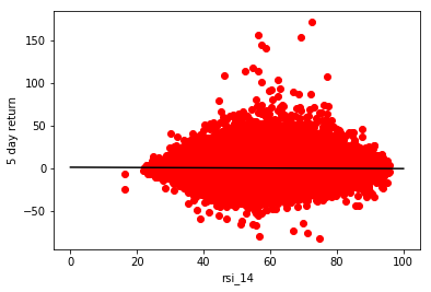
The graph seems to indicate that there is absolutely no correlation between RSI and returns.
Let’s try again with RSI 5 and 1 week returns.
r: -0.04079039357384174, m: -0.009846624341020193, b: 0.8480953908639126
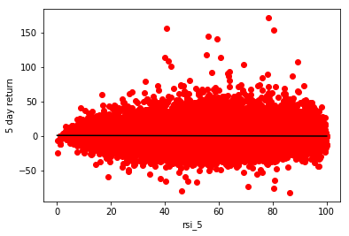
We once again get nothing, but noise.
Statistical Insights
Ok, clearly predicting returns given the value of RSI will not work. How about we group the data by its RSI value. Since RSI ranges from 0 to 100, we can use 10 bins of size 10. I decided to use RSI 5 for the rest of this analysis since that way I am using 1 week of data to predict the next week’s returns. The results are similar for RSI 2 and RSI 14 anyways, but RSI 5 seemed more appropriate.
def get_bins(n,min_,max_):
    return pd.IntervalIndex.from_tuples([(a*(max_-min_)/n+min_, \
    	(a+1)*(max_-min_)/n+min_) for a in range(n)])

bins_by_indicator = {
    'rsi_5': get_bins(10,0,100),
    'rsi_14' : get_bins(10,30,100),
    'wr_5' : get_bins(10,0,100),
    'cci_5': get_bins(10,-200,200)
}

def get_grouped_data(data, indicator, ret_names):
    bins = bins_by_indicator[indicator]
    data_grouped = data.groupby(pd.cut(data[indicator],bins))
    return data_grouped[ret_names]

data_grouped = get_grouped_data(data_plt, 'rsi_5', ret_names)
Now let’s look at the mean, std deviation, and count for each bin.
m = data_grouped.mean().rename(columns={ret_names[0]:'mean'})
s = data_grouped.std().rename(columns={ret_names[0]:'std'})
c = data_grouped.count().rename(columns={ret_names[0]:'count'})
print(pd.concat([m,s,c],axis=1))
                   mean       std   count
rsi_5
(0.0, 10.0]    1.065934  4.558964    1934
(10.0, 20.0]   0.809773  4.528378   28463
(20.0, 30.0]   0.671988  4.516538   95656
(30.0, 40.0]   0.490236  4.497505  187743
(40.0, 50.0]   0.368746  4.486767  280868
(50.0, 60.0]   0.276761  4.432265  347528
(60.0, 70.0]   0.194753  4.309676  362742
(70.0, 80.0]   0.147585  4.177146  306616
(80.0, 90.0]   0.039340  4.088299  185852
(90.0, 100.0] -0.072874  4.267614   44865
Relative to the means, the standard deviation is really high, which explains the difficulty in predicting returns given RSI. However, there is a clear pattern in the means for each bin. Let’s graph it.
data_means = data_grouped.mean()
ax = data_means.plot(style='.',figsize=(15,6), xlim=(-0.1,9.1), legend=True)
ax.set_ylabel("mean returns")

plt.show()
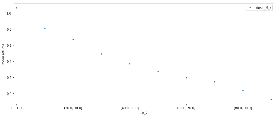
It looks like RSI does actually predict the mean returns. Since the standard deviation is so high, we are obliged to run some testing to determine whether these means are actually statistically different, or if it is just by chance.
We can run a two-sample t-test on pairs of means from consecutive bins. For example, we compare means in bin (0,10] vs. (10,20], (10,20] vs (20,30], and so on. Note that I’ve explained the issues with a t-test on this data a little further below.
For those unfamiliar with a t-test, the idea is that we have a null-hypothesis (i.e. our assumption) that the mean of the two samples is the same, and we are testing the validity of this. When we assume the means are equal, we know the distribution of something called the t-statistic (a function of the data), which follows a t-distribution. If we calculate the value the of the t-statistic with our data, we can determine where on the t-distribution it falls, and therefore the probability (the p-value) of it obtaining that value, given our assumption that the means are equal. If the p-value is less than 0.05 (this is a standard threshold used in statistics), then we can reject the null-hypothesis, i.e. determine that there is a statistically significant difference between the two means.
#idx1 and idx2 are the bins we want to test against each other
def run_two_sample_t_test(data_grouped, idx1, idx2):
    bins = list(data_grouped.indices)
    s1 = data_grouped.get_group(bins[idx1])
    s2 = data_grouped.get_group(bins[idx2])

    t_stat, p_value = stats.ttest_ind(s1,s2,equal_var=False)
    print('t-stat:{}    df:{}    p-value:{}' \
    	.format(t_stat,len(s1)+len(s2)-2, p_value))

for i in range(9):
    run_two_sample_t_test(data_grouped, i, i+1)
t-stat:[ 2.39213099]    df:30395     p-value:[ 0.01683433]
t-stat:[ 4.50919492]    df:124117    p-value:[ 6.52325558e-06]
t-stat:[ 10.14445619]   df:283397    p-value:[ 3.55694993e-24]
t-stat:[ 9.07009213]    df:468609    p-value:[ 1.19430358e-19]
t-stat:[ 8.12396478]    df:628394    p-value:[ 4.52043840e-16]
t-stat:[ 7.90107083]    df:710268    p-value:[ 2.76911054e-15]
t-stat:[ 4.53643952]    df:669356    p-value:[ 5.72219870e-06]
t-stat:[ 8.9327637]    	df:492466    p-value:[ 4.17199913e-19]
t-stat:[ 5.0392082]    	df:230715    p-value:[ 4.68690463e-07]
Based on the p-values, the means are significantly different between all pairs of bins. The first two bins have a relatively high p-value compared to the other tests, which can be explained by the fact that the first bin has a smaller sample size.
Note that for the t-tests we did not assume that the data is normally distributed in each group, just that the means are normally distributed, which is true for large enough sample sizes like ours by the Central Limit Theorem (CLT). The main issue with this test is that our data is not independent for various reasons (and hence the CLT doesn’t hold). I believe that this t-test is still valuable since the p-values we got for most of our tests are so low, that even a large adjustment in standard deviation and degrees of freedom to compensate for some of the dependence will yield low p-values. Of course, this still doesn’t mean that our tests are valid, but the clear pattern in decreasing means as RSI increases does suggest a significant difference in means (even if we can’t statistically prove it).
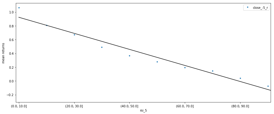
We can also run a linear regression on the mean returns vs. RSI 5 to put the strong relation into perspective.
r: -0.9796442703777255, m: -0.11662270769899107, b: 0.9240265419040458
Returns on Different Holding Periods
We determined that there is a strong correlation between mean 1 week returns and RSI 5 value. What about 2 day returns or 10 day returns?
ret_days = [1,2,3,4,5,6,7,8,9,10]
ret_names = ['close_-{}_r'.format(d) for d in ret_days]
indicators = ['rsi_5']
data = load_data(indicators, ret_days, ret_names)

data_plt = clean_data(data)
data_grouped = get_grouped_data(data_plt, 'rsi_5', ret_names)
data_means = data_grouped.mean()

ax = data_means.plot(figsize=(15,6), xlim=(-0.1,9.1), legend=True)
ax.set_ylabel("mean returns")
plt.show()
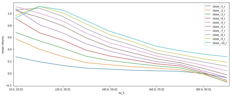
For this graph I’ve changed from a scatter plot to a line graph so it’s obvious which points belong to which return period. As you can see, the results are pretty consistent for each return period, except at the extreme ends of RSI values. This further solidifies our conclusion that RSI can predict mean short-term returns.
Practically Using this Information
We’ve found that the mean returns can be predicted, but the variance of each investment is extremely high. When investing, we have two goals: to generate returns and to minimize return variance. If we invest in one stock at a time, then we lose/earn a lot each time, and would achieve a standard deviation in return equal to about (when looking at 1 week returns). If we invest in 100 stocks at a time, we would achieve a standard deviation of about each time we invest. Now, of course, this assumes that returns given RSI are uncorrelated, which is most likely not true, meaning that the true standard deviation of 1 week returns is probably higher.
Caveats
It is important to note that this analysis was done on current members of the S&P 500 and therefore, there is survivorship bias. In the future I will make a more comprehensive analysis that accounts for the members of the S&P 500 at any given time.
Backtesting
The next step is to backtest our model and see what kind of results we get. This will be detailed in a later post.