Backtesting an RSI Strategy
Goal
Last time we showed some promising statistical results regarding RSI and its ability to predict mean returns. Now we want to show that these results can be practically used to generate better returns than the market. Since my previous post primarily focused on RSI 5 (with price above SMA 100), we will also be backtesting using RSI 5.
The Setup
Before I go into any results, we have to decide how exactly we’re going to set up our backtest. I decided to use a simple model where, once each week, we will identify stocks with RSI values below a certain threshold, hold them for a week, then repeat. Since low RSI correlates with higher mean returns, we want to choose as low of an RSI threshold as possible, but high enough so that we have enough stocks to invest in every week in order to minimize our volatility (as I argued in my last post). A good number of stocks to hold would be 20, and out of 3 million data points I looked at over 20 years in the S&P 500, only about 4% of the time was the RSI 5 < 30 and stock price above its SMA 100, which equates to an average of 20 stocks at a time satisfying these conditions (since 4% of 500 is 20). If we choose a lower RSI threshold of 20, then we would only expect to be invested in about 5 stocks at a time, which is much too low.
Each week we will split our portfolio among the stocks with RSI 5 < 30 evenly, with the constraint that we will not invest more than 5% in any one stock, so as to reduce our exposure to a single stock. I chose 5% since it would be the weight of a stock if we invested in 20 stocks at once.
import pandas as pd
import matplotlib.pyplot as plt
import numpy as np
from scipy import stats
from stockstats import StockDataFrame as Sdf # https://pypi.org/project/stockstats/
import os

# backtesting library
# note if you download the anaconda ffn distribution, it will not work correctly
# you need to download the library locally from https://github.com/pmorissette/ffn
import sys
sys.path.insert(0, r'D:\Libraries\ffn-master')
import ffn
import bt

# data source
# your data source will be different
# recommend using datareader from https://github.com/pydata/pandas-datareader
hist_folder = r'D:\S&P 500\\'
tickers = [ticker.replace('.csv','') for ticker in os.listdir(hist_folder)]
def get_hist_prices(ticker):
    return pd.read_csv(hist_folder+ticker+".csv",index_col=0)

# load ticker and indicator data
sma,sma_days = 'close_100_sma',100
def load_data(indicators):
    prices = pd.DataFrame(columns=tickers)
    indicator_data = [pd.DataFrame(columns=tickers) for indicator in indicators]
    sma_data = pd.DataFrame(columns=tickers)
    for ticker in tickers:
        print(ticker)
        ticker_data = Sdf.retype(get_hist_prices(ticker))

        prices[ticker] = ticker_data['close']
        for i,indicator in enumerate(indicators):
            indicator_data[i][ticker] = ticker_data[indicator]
        sma_data[ticker] = ticker_data[sma]

    prices.index = pd.to_datetime(prices.index,format='%Y%m%d')
    sma_data.index = pd.to_datetime(sma_data.index,format='%Y%m%d')
    prices.fillna(inplace=True, method='pad')
    for i in range(len(indicator_data)):
        indicator_data[i].index = pd.to_datetime(indicator_data[i].index,format='%Y%m%d')

    return prices, indicator_data, sma_data

indicators = ['rsi_5']
prices, indicator_data, sma_data = load_data(indicators)

# calculate weights for backtesting
# if a ticker statisfies the RSI 5 and SMA 100 condition, then set its weight to 1 on that day
def calculate_weights(indicators, indicator_data, threshold, hold_period):
    weights = [None for indicator in indicators]
    for i,indicator in enumerate(indicators):
        weights[i] = indicator_data[i].copy()
        condition = (weights[i] <= threshold) & (sma_data < prices) # hold condition
        weights[i][condition] = 1
        weights[i][~condition] = 0

    return weights

# split weights evenly among all stocks with weight 1 on a given day
def split_weights(weights, max_weight=0.05):
    out_weights = []

    for weight_df in weights:
        weight_tot = weight_df.sum(axis=1)
        scaled = weight_df.div(weight_tot,axis=0)
        scaled = np.minimum(scaled,max_weight)
        out_weights.append(scaled)
    return out_weights


weights = calculate_weights(indicators, indicator_data, 30, None)
weights = split_weights(weights)
We can take a look at our total weights to see how much of our portfolio is invested at a time.
weight_tot = weights[0].sum(axis=1) # count total weights per day
counts = weights[0].fillna(0).astype(bool).sum(axis=1) # count number of stocks per day
plt.figure(figsize = (20,10))
plt.subplot(2, 1, 1)
plt.bar(weight_tot.index, weight_tot,width=5) # width=5 so we can see the bars
plt.subplot(2, 1, 2)
plt.bar(counts.index,counts,width=5)
plt.show()

# print average portfolio weight and the average number of stocks
print(weight_tot.mean())
print(counts.mean())
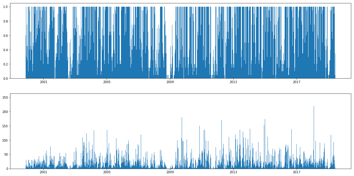
0.5513395575400865
18.592652729855896
This tells us we are invested about 55% on average (and 18 stocks on average confirms our prediction of 20), but it fluctuates quite a bit.
Backtesting
Now we can backtest the weights we’ve set up to see some results.
# simple backtest to test long-only allocation
def long_only_equal_weight():
    s = bt.Strategy('current_sp500', [bt.algos.RunOnce(),
                           bt.algos.SelectAll(),
                           bt.algos.WeighEqually(),
                           bt.algos.Rebalance()])
    return bt.Backtest(s, prices)

# generate the buy and hold benchmark for stocks currently in S&P 500
benchmark = long_only_equal_weight()

# run our backtest on the given weights
def run_backtest(num_periods, weights,name):
    s = bt.Strategy(name,
                  [bt.algos.WeighTarget(weights),
                   bt.algos.RunEveryNPeriods(num_periods),
                   bt.algos.Rebalance()])
    return bt.Backtest(s,prices)

res = bt.run(run_backtest(5,weights[0],'{} day return'.format(5)), benchmark)
res.plot()
plt.show()
res.display()
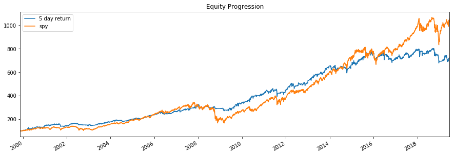 With this strategy we acheived a return of 10.62% per year with a max drawdown of 17.39%.
I benchmarked this strategy against an equally weighted portfolio of current S&P 500 members to help account for survivorship bias. Of course this is not the same as working with the actual historical constituents of the index, but it allows us to compare our results.
Full Results (click here)
Stat                 5 day return    current_sp500
-------------------  --------------  --------------
Start                1999-11-17      1999-11-17
End                  2019-06-20      2019-06-20
Risk-free rate       0.00%           0.00%

Total Return         621.60%         957.09%
Daily Sharpe         0.85            0.72
Daily Sortino        1.35            1.15
CAGR                 10.62%          12.79%
Max Drawdown         -17.39%         -51.45%
Calmar Ratio         0.61            0.25

MTD                  4.04%           6.77%
3m                   1.97%           6.38%
6m                   1.43%           21.88%
YTD                  3.82%           20.19%
1Y                   -7.88%          4.77%
3Y (ann.)            -1.34%          10.93%
5Y (ann.)            2.36%           10.43%
10Y (ann.)           10.02%          17.61%
Since Incep. (ann.)  10.62%          12.79%

Daily Sharpe         0.85            0.72
Daily Sortino        1.35            1.15
Daily Mean (ann.)    10.95%          13.96%
Daily Vol (ann.)     12.95%          19.45%
Daily Skew           -0.08           -0.18
Daily Kurt           10.68           7.64
Best Day             6.94%           11.06%
Worst Day            -7.95%          -9.87%

Monthly Sharpe       1.05            0.89
Monthly Sortino      1.89            1.54
Monthly Mean (ann.)  10.71%          13.34%
Monthly Vol (ann.)   10.19%          14.99%
Monthly Skew         -0.40           -0.73
Monthly Kurt         2.43            2.00
Best Month           11.60%          11.50%
Worst Month          -11.46%         -19.81%

Yearly Sharpe        0.82            0.79
Yearly Sortino       3.19            1.66
Yearly Mean          11.11%          13.80%
Yearly Vol           13.49%          17.52%
Yearly Skew          0.28            -1.30
Yearly Kurt          0.40            1.83
Best Year            43.49%          36.40%
Worst Year           -11.62%         -34.76%

Avg. Drawdown        -2.03%          -2.31%
Avg. Drawdown Days   29.86           23.70
Avg. Up Month        2.39%           3.65%
Avg. Down Month      -2.13%          -3.28%
Win Year %           80.00%          85.00%
Win 12m %            80.89%          81.78%
Backtesting over Different Holding Periods
In my last post, I showed that RSI predicted the mean returns for holding periods other than 1 week as well. It would be a good idea to see how these different holding periods do in a backtest. We will use the same setup as above.
backtests = []
for i in range(1,11): # backtest holding periods 1..10 days
    backtests.append(run_backtest(i,weights[0],'{} day return'.format(i)))
res = bt.run(*backtests, benchmark)
res.plot()
plt.show()
res.display()
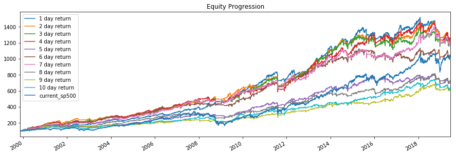
Multiple Holding Period Results
Stat 1 day return 2 day return 3 day return 4 day return 5 day return 6 day return 7 day return 8 day return 9 day return 10 day return current_sp500
------------------- -------------- -------------- -------------- -------------- -------------- -------------- -------------- -------------- -------------- --------------- ---------------
Start 1999-11-17 1999-11-17 1999-11-17 1999-11-17 1999-11-17 1999-11-17 1999-11-17 1999-11-17 1999-11-17 1999-11-17 1999-11-17
End 2019-06-20 2019-06-20 2019-06-20 2019-06-20 2019-06-20 2019-06-20 2019-06-20 2019-06-20 2019-06-20 2019-06-20 2019-06-20
Risk-free rate 0.00% 0.00% 0.00% 0.00% 0.00% 0.00% 0.00% 0.00% 0.00% 0.00% 0.00%
Total Return 1161.70% 1155.18% 1098.56% 1166.23% 621.60% 938.21% 1096.71% 629.10% 510.55% 537.50% 957.09%
Daily Sharpe 1.06 1.07 1.07 1.08 0.85 1.04 1.10 0.88 0.82 0.79 0.72
Daily Sortino 1.68 1.70 1.71 1.72 1.35 1.67 1.76 1.40 1.28 1.26 1.15
CAGR 13.82% 13.79% 13.52% 13.84% 10.62% 12.69% 13.51% 10.67% 9.68% 9.92% 12.79%
Max Drawdown -19.81% -18.12% -17.94% -18.17% -17.39% -14.71% -17.32% -21.37% -16.00% -25.74% -51.45%
Calmar Ratio 0.70 0.76 0.75 0.76 0.61 0.86 0.78 0.50 0.60 0.39 0.25
MTD 3.64% 3.58% 3.26% 4.97% 4.04% 3.07% 3.63% 5.44% 1.01% 5.03% 6.77%
3m -1.85% -3.45% -2.09% 1.04% 1.97% -1.02% -1.46% 0.04% -1.81% -3.03% 6.38%
6m -3.15% -3.37% -1.00% -0.33% 1.43% -0.16% -2.78% -0.55% 0.55% -4.22% 21.88%
YTD -0.16% -0.98% 0.48% 2.55% 3.82% 1.43% -2.39% 0.38% -0.18% -3.33% 20.19%
1Y -13.84% -10.63% -9.12% -9.00% -7.88% -3.59% -9.13% -4.48% -6.84% -8.70% 4.77%
3Y (ann.) -0.79% 0.96% -0.45% 0.34% -1.34% -0.31% 4.43% 5.57% 7.12% 3.10% 10.93%
5Y (ann.) 0.87% 0.48% 0.03% 2.48% 2.36% 0.41% 1.95% 5.15% 6.63% 7.63% 10.43%
10Y (ann.) 9.98% 9.18% 9.86% 10.23% 10.02% 9.64% 9.52% 10.28% 10.90% 11.22% 17.61%
Since Incep. (ann.) 13.82% 13.79% 13.52% 13.84% 10.62% 12.69% 13.51% 10.67% 9.68% 9.92% 12.79%
Daily Sharpe 1.06 1.07 1.07 1.08 0.85 1.04 1.10 0.88 0.82 0.79 0.72
Daily Sortino 1.68 1.70 1.71 1.72 1.35 1.67 1.76 1.40 1.28 1.26 1.15
Daily Mean (ann.) 13.81% 13.77% 13.50% 13.81% 10.95% 12.71% 13.44% 10.93% 10.01% 10.32% 13.96%
Daily Vol (ann.) 12.98% 12.85% 12.60% 12.83% 12.95% 12.17% 12.17% 12.42% 12.24% 13.00% 19.45%
Daily Skew -0.36 -0.30 -0.07 -0.26 -0.08 -0.10 -0.22 -0.15 -0.22 -0.05 -0.18
Daily Kurt 9.45 8.79 7.46 9.92 10.68 7.72 8.07 9.42 9.25 11.54 7.64
Best Day 5.99% 5.95% 5.99% 6.18% 6.94% 5.14% 5.50% 6.94% 5.85% 6.95% 11.06%
Worst Day -8.36% -7.95% -5.54% -7.95% -7.95% -5.42% -6.60% -7.48% -7.21% -7.95% -9.87%
Monthly Sharpe 1.31 1.25 1.27 1.25 1.05 1.29 1.29 1.06 1.04 1.00 0.89
Monthly Sortino 2.28 2.22 2.22 2.21 1.89 2.68 2.49 2.06 2.03 1.72 1.54
Monthly Mean (ann.) 13.58% 13.66% 13.34% 13.67% 10.71% 12.47% 13.28% 10.70% 9.72% 10.02% 13.34%
Monthly Vol (ann.) 10.36% 10.89% 10.51% 10.92% 10.19% 9.70% 10.27% 10.08% 9.36% 10.04% 14.99%
Monthly Skew -0.98 -0.71 -0.83 -0.67 -0.40 0.00 -0.20 0.26 0.06 -0.65 -0.73
Monthly Kurt 3.28 2.42 2.92 2.50 2.43 1.37 2.90 3.68 1.45 2.61 2.00
Best Month 8.44% 12.41% 10.45% 12.33% 11.60% 11.21% 12.25% 14.52% 9.79% 9.67% 11.50%
Worst Month -13.64% -12.14% -12.08% -11.13% -11.46% -8.80% -11.21% -8.68% -7.60% -10.93% -19.81%
Yearly Sharpe 0.90 0.83 0.81 0.85 0.82 0.91 0.87 0.75 0.75 0.73 0.79
Yearly Sortino 4.52 7.70 6.01 4.17 3.19 6.69 16.91 2.73 3.30 2.17 1.66
Yearly Mean 14.06% 14.14% 14.05% 14.25% 11.11% 12.94% 13.83% 10.91% 10.06% 10.52% 13.80%
Yearly Vol 15.66% 17.05% 17.37% 16.82% 13.49% 14.26% 15.82% 14.62% 13.40% 14.40% 17.52%
Yearly Skew 0.94 2.22 2.02 1.15 0.28 1.39 1.85 0.55 1.61 0.07 -1.30
Yearly Kurt 1.94 7.23 6.50 2.99 0.40 3.51 5.05 0.97 5.02 0.31 1.83
Best Year 56.92% 73.05% 72.92% 63.83% 43.49% 56.34% 65.34% 47.34% 53.06% 37.75% 36.40%
Worst Year -13.77% -7.93% -9.83% -13.68% -11.62% -6.06% -2.76% -17.70% -10.96% -19.86% -34.76%
Avg. Drawdown -1.65% -1.68% -1.73% -1.72% -2.03% -1.69% -1.54% -1.92% -1.85% -1.92% -2.31%
Avg. Drawdown Days 19.04 19.65 22.48 21.91 29.86 24.63 19.90 28.03 28.35 27.30 23.70
Avg. Up Month 2.58% 2.67% 2.55% 2.64% 2.39% 2.41% 2.48% 2.25% 2.15% 2.32% 3.65%
Avg. Down Month -2.28% -2.39% -2.43% -2.34% -2.13% -1.78% -1.93% -2.01% -1.93% -1.99% -3.28%
Win Year % 80.00% 80.00% 85.00% 85.00% 80.00% 85.00% 85.00% 75.00% 85.00% 80.00% 85.00%
Win 12m % 87.56% 88.44% 84.00% 89.33% 80.89% 84.44% 87.56% 79.11% 83.56% 82.67% 81.78%
The shorter holding periods seem to do much better than the longer holding periods on average, but there is some variance in the results (i.e. 7 days doing better than expected, and 5 days doing worse). This overall result can be explained by the fact that the holding period graph in my previous post showed that even though the mean returns increase as the holding period increases, that size of that increase gets smaller, which implies that the average return per day actually decreases as the holding period increases. This explains why the overall return above is higher for shorter holding periods.
Backtesting Different RSI Values
The idea behind using RSI as a predictor for mean returns is that low RSI values correspond to higher mean returns, but we need to pick a lot of stocks with low RSI values in order to realize these returns with minimal drawdown. If we pick a low RSI threshold, then there are not enough stocks to minimize the drawdowns, and if we pick a high RSI threshold, then we pick a portfolio with lower mean returns, meaning smaller returns for the risk we take. Below, we backtest on RSI thresholds from 10-70 in increments of 5 and use the MAR ratio (labelled as Calmar below) and Sharpe ratio as ways to compare our results.
threshold_weights = []
for i in range(2,15):
    w = calculate_weights(indicators, indicator_data, 5*i, None)
    threshold_weights += split_weights(w,max_weight=0.05) # Assign fixed weight to each stock

backtests = []
for i in range(len(threshold_weights)):
    backtests.append(run_backtest(5,threshold_weights[i], 'rsi threshold {}'.format(5*(i+2))))
res = bt.run(*backtests)
res.display()
Stat                 rsi threshold 10    rsi threshold 15    rsi threshold 20    rsi threshold 25    rsi threshold 30    rsi threshold 35    rsi threshold 40    rsi threshold 45    rsi threshold 50    rsi threshold 55    rsi threshold 60    rsi threshold 65    rsi threshold 70
-------------------  ------------------  ------------------  ------------------  ------------------  ------------------  ------------------  ------------------  ------------------  ------------------  ------------------  ------------------  ------------------  ------------------
Start                1999-11-17          1999-11-17          1999-11-17          1999-11-17          1999-11-17          1999-11-17          1999-11-17          1999-11-17          1999-11-17          1999-11-17          1999-11-17          1999-11-17          1999-11-17
End                  2019-06-20          2019-06-20          2019-06-20          2019-06-20          2019-06-20          2019-06-20          2019-06-20          2019-06-20          2019-06-20          2019-06-20          2019-06-20          2019-06-20          2019-06-20
Risk-free rate       0.00%               0.00%               0.00%               0.00%               0.00%               0.00%               0.00%               0.00%               0.00%               0.00%               0.00%               0.00%               0.00%

Total Return         5.38%               52.03%              173.33%             395.69%             621.60%             1074.12%            1248.39%            1541.55%            1562.16%            1446.65%            1257.05%            959.82%             737.49%
Daily Sharpe         0.23                0.60                0.78                0.86                0.85                0.92                0.92                0.95                0.93                0.90                0.85                0.78                0.70
Daily Sortino        0.35                0.89                1.20                1.35                1.35                1.47                1.47                1.51                1.49                1.44                1.36                1.23                1.10
CAGR                 0.27%               2.16%               5.27%               8.51%               10.62%              13.40%              14.20%              15.36%              15.43%              15.00%              14.24%              12.81%              11.46%
Max Drawdown         -2.99%              -10.45%             -15.53%             -16.47%             -17.39%             -26.15%             -40.60%             -43.52%             -47.03%             -48.40%             -53.70%             -58.47%             -63.19%
Calmar Ratio         0.09                0.21                0.34                0.52                0.61                0.51                0.35                0.35                0.33                0.31                0.27                0.22                0.18
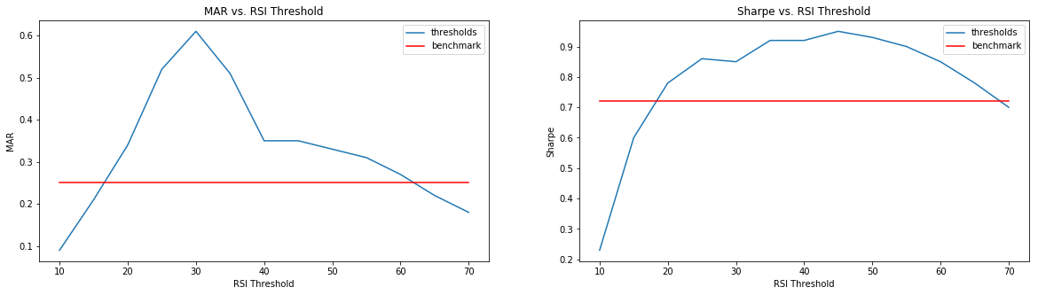
As you can see, there is an optimum RSI threshold that maximizes the MAR ratio, and a different optimum RSI threshold that maximized the Sharpe ratio. The results I have are achieved using a ‘max_weight’ parameter of 0.05 when I split the weights. This parameter can be optimized for each RSI threshold in order to increase the MAR and Sharpe ratios. However, the purpose of these results is just to show that the optimum results are not acheived by a very low or very high RSI threshold for the reasons I stated above.
Conclusion
Our goal was to show that we could use our statistical RSI results to construct a portfolio that generates above market returns. In the end, we found that an RSI threshold of 30-40 generated the best results, but we also showed that even though our statistics showed that RSI thresholds of 10 and 20 were theoretically better, that they did not perform as well as thresholds of 30-40. We can easily explain this by the fact that using small thresholds prevents us from diversifying since there are simply not enough stocks with such low RSIs at any given time. But it is important to understand real world limitations like these when trying to take theoretical models and apply them practically.